Donor targeting for NonProfit campaign
The objective of this post is to show a complete, concrete and concise business data science use-case. We will go from MySQL data extraction to customer scoring using R.
Context: Our main dataset is a table indicating if a donor made a donation in response of a recent marketing campaign. If a donation has been made, we have the specific amount and date of the donation.
From that, and having access to other information in the main SQL database of the NonProfit organization, we want to be able to predict the donors most likely to give for a future donation campaign.
In the end we can focus on targeting the high value prospects, to maximize the donation campaign margin.
Data overview
The donation table we are working out has the following variables:
- contact_id: Unique identifier of a donor, can be used to link with other tables from company’s database
- donation: Did the contact make a donation ?
- amount: If a donation has been made, give its specific amount
- act_date: If a donation has been made, give its specific date
In addition to that table we have access to the rest of the Organization database. Here is a schema of the remaining tables:
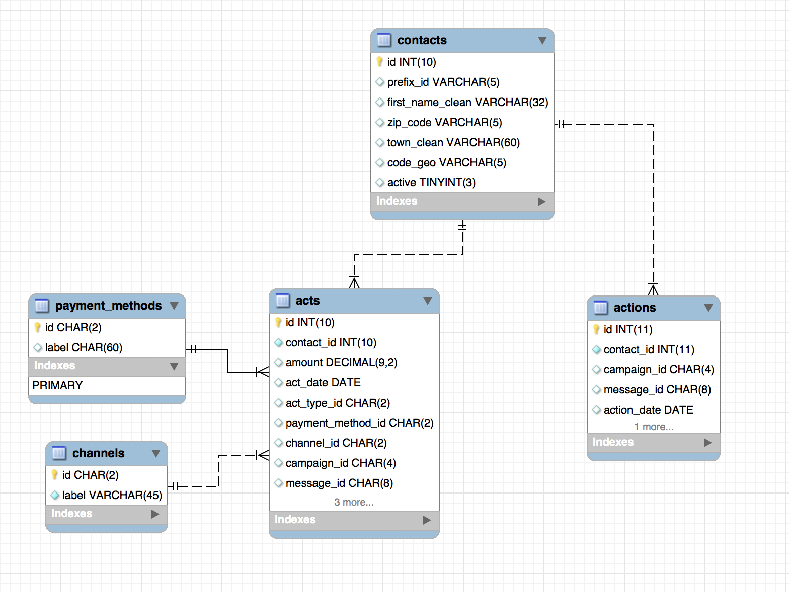
The contact table gives us more donor information, like geolocation or if a person is considered active.
The acts table contains a history of all donations made to the NonProfit organization since its existence and its details: amount, date, type of payment, how the contact has been reached, is the donation in response to a campaign.
The actions table contains a history of all actions from the NonProfit organization. An action consists in reaching a contact, like sending a mail.
Get what we need from MySQL to R
Now that we understand what data we are dealing with, we need to extract it from the database. We will use R for data munging and modeling, so we need to connect to MySQL from R. To do so, beside from having R and MySQL, we need the RODBC package.
We load the package and establish the connection with the following code:
library(RODBC)
db = odbcConnect("mysqlodbc", uid="ID", pwd="PASSWORD")
We can then define our query directly in R and import the result as a dataframe. First let’s import the main dataset, donation
query = "SELECT * FROM donation"
donation = sqlQuery(db, query)

library(dplyr)
We can then extract, for each table of the database, the indicators we want as predictors for modeling. It is interesting to do a large part of our manipulation directly in MySQL while possible, for the sake of efficiency.
From the acts table (entire donations history), we can use amount to have an average donation amount for each donor, and count the frequency of donation for each donor. We can also use act_date to look at how recent is the last donation of a donor, and how long since the first donation. Finally, we can look if a donor has made donation in the past year.
query = "
    SELECT
        a.contact_id,
        AVG(a.amount) AS 'avg_amount',
        COUNT(a.amount)  AS 'frequency',
        DATEDIFF(20170622, MAX(a.act_date)) / 365 AS 'recency',
        DATEDIFF(20170622, MIN(a.act_date)) / 365 AS 'seniority',
        IF(c.counter IS NULL, 0, 1) AS 'loyal'
    FROM acts a
    LEFT JOIN (
        SELECT
            contact_id,
            COUNT(amount) AS counter
        FROM acts
        WHERE
            (act_date >= 20160622) AND
            (act_date < 20170622) AND
            (act_type_id = 'DO')
        GROUP BY contact_id
    ) AS c
    ON c.contact_id = a.contact_id
    WHERE
        (act_type_id = 'DO') AND
        (act_date < 20170622)
    GROUP BY 1
"
acts_indicators = sqlQuery(db, query)
From the actions table (entire contact reaching history), we can obtain a notion of responsiveness to campaign for each donor. To do so we count how many times a donor has been reached, and divide by how many times that donor made a donation linked to a campaign_id. We only look on the past 5 years to obtain, in case a donor has been very responsive in the past but changed its behavior after a while.
query = "
    SELECT
        a.contact_id,
        b.response  / a.nb_sollicitations AS 'responsiveness'
    FROM (
        SELECT
            actions.contact_id,
            count(actions.contact_id) AS 'nb_sollicitations'
        FROM actions
        WHERE
            actions.action_date >= 20120622
        GROUP BY actions.contact_id
    ) AS a
    LEFT JOIN (
        SELECT
            acts.contact_id,
            count(acts.campaign_id) AS 'response'
        FROM acts
        WHERE
            acts.act_type_id = 'DO' AND
            acts.act_date >= 20120622 AND
            acts.campaign_id IS NOT NULL
        GROUP BY acts.contact_id
    ) AS b
    ON a.contact_id = b.contact_id
"
actions_indicators = sqlQuery(db, query)
Finally from the contacts table prefix_id is interesting because indicating the donor’s title, and zip_code can be used to check the area if we keep only the 2 first digits. active can be kept as such.
query = "
    SELECT
        contacts.id,
        contacts.prefix_id,
        SUBSTRING(contacts.zip_code,1, 2) 				AS 'zip',
        contacts.active
    FROM contacts
"
contacts_indicators = sqlQuery(db, query)
colnames(contacts_indicators)[1] <- "contact_id"
A bit of data munging
We have everything in R, now let’s make a unique dataset out of our dataframes.
Normally we would prefer to join directly in MySQL as well, but the dataset beeing relatively small (62 000 donations) we can do it in R.
dataset = merge(x = donation, y = acts_indicators, by = "contact_id", all.x = TRUE)
dataset = merge(x = dataset, y = actions_indicators, by = "contact_id", all.x = TRUE)
dataset = merge(x = dataset, y = contacts_indicators, by = "contact_id", all.x = TRUE)
Even if we changed the data with the SQL queries, some features still need to be modified before modeling.
summary(dataset)
   contact_id         donation          amount            act_date
 Min.   :    106   Min.   :0.0000   Min.   :    2.00   Min.   :2017-06-26
 1st Qu.: 885292   1st Qu.:0.0000   1st Qu.:   20.00   1st Qu.:2017-07-06
 Median : 954649   Median :0.0000   Median :   30.00   Median :2017-07-10
 Mean   : 905617   Mean   :0.1043   Mean   :   49.16   Mean   :2017-07-17
 3rd Qu.:1010400   3rd Qu.:0.0000   3rd Qu.:   50.00   3rd Qu.:2017-07-21
 Max.   :1523424   Max.   :1.0000   Max.   :10000.00   Max.   :2017-10-12
                                    NA's   :55472      NA's   :55472
   avg_amount         frequency          recency          seniority
 Min.   :    0.03   Min.   :  1.000   Min.   : 0.0027   Min.   : 0.0164
 1st Qu.:   20.70   1st Qu.:  2.000   1st Qu.: 0.4795   1st Qu.: 2.5151
 Median :   30.00   Median :  5.000   Median : 0.6521   Median : 5.5863
 Mean   :   43.14   Mean   :  9.005   Mean   : 1.2922   Mean   : 7.1331
 3rd Qu.:   48.46   3rd Qu.: 12.000   3rd Qu.: 1.5425   3rd Qu.:10.5205
 Max.   :27875.00   Max.   :132.000   Max.   :25.4932   Max.   :47.2904
 NA's   :2646       NA's   :2646      NA's   :2646      NA's   :2646
     loyal        responsiveness  prefix_id         zip            active
 Min.   :0.0000   Min.   :0.021   AU  :   52   75     : 2604   Min.   :0.000
 1st Qu.:0.0000   1st Qu.:0.105   DR  :   28   59     : 2437   1st Qu.:1.000
 Median :1.0000   Median :0.147   MLLE: 8919   13     : 2128   Median :1.000
 Mean   :0.6411   Mean   :0.198   MME :39638   92     : 1949   Mean   :0.993
 3rd Qu.:1.0000   3rd Qu.:0.242   MMME: 3132   06     : 1823   3rd Qu.:1.000
 Max.   :1.0000   Max.   :4.500   MR  :10023   (Other):50972   Max.   :1.000
 NA's   :2646     NA's   :4602    NA's:  136   NA's   :   15
We keep prefix as one hot encoded features, excluding the less frequent options that are MMME, AU and DR.
dataset$MR = ifelse(dataset$prefix_id == 'MR', 1, 0)
dataset$MME = ifelse(dataset$prefix_id == 'MME', 1, 0)
dataset$MLLE = ifelse(dataset$prefix_id == 'MLLE', 1, 0)
We do the same for the Zip, but keeping only the most present area, 75.
dataset$area_is_75 = ifelse(dataset$zip == '75', 1, 0)
We can see with the above summary of the dataset that there is NAs. Those should be replaced or could cause issue during modeling.
dataset$amount[is.na(dataset$amount)] = 0
dataset$avg_amount[is.na(dataset$avg_amount)] = 0
dataset$frequency[is.na(dataset$frequency)] = 0
dataset$recency[is.na(dataset$recency)] = 100
dataset$seniority[is.na(dataset$seniority)] = 0
dataset$loyal[is.na(dataset$loyal)] = 0
dataset$responsiveness[is.na(dataset$responsiveness)] = 0
Perfect ! We now keep only the features we want:
dataset = dataset %>% select(c(donation, amount, avg_amount, frequency,
                               recency, seniority, loyal, responsiveness,
                               MR, MME, MLLE, area_is_75))
Finally, we split our dataset between training and testing set to assess the performance we could have on new data.
library(caTools)

spl = sample.split(dataset$donation, 0.8)
training = subset(dataset, spl=TRUE)
testing = subset(dataset, spl=FALSE)
Here comes machine learning
The main goal is to be able to target high value potential donors from the information we have. How do we do that? We use customer scoring.
Meaning, we want to attribute to each donor a score relative to its potential value. Here, we will have a score depending on the probability that a donor will make a donation, and the amount of the potential donation.
That is why we will fit not one but two models:
- A discrete model, to obtain the probability of a donation for a donor
- A continuous model, to obtain the value of the potential donation
Let’s get to it, with firstly the donation probability model. We use glm (generalized linear models) of the caret package. For this binary classification problem we use family = binomial.
donation_prob_model = glm(donation ~ . -amount, data = training, family = binomial)
summary(donation_prob_model)
Warning message:
“glm.fit: fitted probabilities numerically 0 or 1 occurred”


Call:
glm(formula = donation ~ . - amount, family = binomial, data = training)

Deviance Residuals:
    Min       1Q   Median       3Q      Max
-4.0050  -0.4784  -0.4031  -0.2562   3.5187

Coefficients:
                 Estimate Std. Error z value Pr(>|z|)
(Intercept)    -3.3832688  0.0711345 -47.562  < 2e-16 ***
avg_amount     -0.0013858  0.0003535  -3.920 8.85e-05 ***
frequency       0.0353026  0.0018016  19.595  < 2e-16 ***
recency        -0.0122077  0.0021925  -5.568 2.58e-08 ***
seniority      -0.0019989  0.0035550  -0.562 0.573927
loyal           0.8614736  0.0401433  21.460  < 2e-16 ***
responsiveness  1.8675279  0.0890663  20.968  < 2e-16 ***
MR             -0.2289867  0.0663817  -3.450 0.000562 ***
MME            -0.0883710  0.0579163  -1.526 0.127050
MLLE           -0.2218428  0.0688422  -3.222 0.001271 **
area_is_75     -0.1029471  0.0724242  -1.421 0.155187
---
Signif. codes:  0 ‘***’ 0.001 ‘**’ 0.01 ‘*’ 0.05 ‘.’ 0.1 ‘ ’ 1

(Dispersion parameter for binomial family taken to be 1)

    Null deviance: 41301  on 61776  degrees of freedom
Residual deviance: 36122  on 61766  degrees of freedom
  (151 observations deleted due to missingness)
AIC: 36144

Number of Fisher Scoring iterations: 7
Interesting to notice, care indicates us (thanks to the P values) that almost all the features we chose are significant for the model. Only seniority, MME and are_is_75 are not.
prob_predictions = predict(donation_prob_model, newdata= testing, type="response")
table(prob_predictions > 0.5, testing$donation)
            0     1
  FALSE 54912  5957
  TRUE    426   482
Looking at the prediction matrix, we can see that our classification model can be considered “securing”. It has a tendency to predict more non-donation than donation. The result are interesting considering the problem we are facing, and the threshold could be modify if the NonProfit is willing to risk more cost for more margin.
Now time to predict the amount of the donations. We use again glm, but this time with family = gaussian that will fit more the distribution of the donation amount.
donation_amount_model = glm(amount ~ . -donation, data = training, family = gaussian)
summary(donation_amount_model)
Call:
glm(formula = amount ~ . - donation, family = gaussian, data = training)

Deviance Residuals:
    Min       1Q   Median       3Q      Max
-1099.6     -5.9     -3.3     -0.4   9864.4

Coefficients:
               Estimate Std. Error t value Pr(>|t|)
(Intercept)    -3.12543    0.95146  -3.285  0.00102 **
avg_amount      0.03945    0.00138  28.589  < 2e-16 ***
frequency       0.33337    0.03153  10.573  < 2e-16 ***
recency         0.03214    0.01049   3.066  0.00217 **
seniority      -0.05409    0.05237  -1.033  0.30164
loyal           2.46809    0.44312   5.570 2.56e-08 ***
responsiveness 11.46837    1.56911   7.309 2.73e-13 ***
MR              0.20088    0.95437   0.210  0.83329
MME             0.29413    0.86266   0.341  0.73314
MLLE            0.62795    0.97092   0.647  0.51779
area_is_75      0.26730    0.94064   0.284  0.77629
---
Signif. codes:  0 ‘***’ 0.001 ‘**’ 0.01 ‘*’ 0.05 ‘.’ 0.1 ‘ ’ 1

(Dispersion parameter for gaussian family taken to be 2200.541)

    Null deviance: 139416698  on 61776  degrees of freedom
Residual deviance: 135918640  on 61766  degrees of freedom
  (151 observations deleted due to missingness)
AIC: 650793

Number of Fisher Scoring iterations: 2
Interestingly again, this model uses less variable than the classification model. Meaning that only the average amount, frequency, recency, loyalty and responsiveness of the donors helps predicting the potential amount of a future donation.
amount_predictions = predict(donation_amount_model, newdata= testing)
Scoring for targeting
We can then combine the predictions of the two models to obtain our donor scores:
scores = prob_predictions * amount_predictions
Here we are! We obtain for each new donor, a score depending on the probability of donation and the amount of that donation.
This method is really useful as it permits to judge the risk of investment for a given donor in a new campaign. If the cost of reaching one donor is 2€, the the NonProfit should target only donors with a score above 2 to cover the investment.
Of course, the margin could be improve by developing the feature engineering even more, or by improving the model trying other methods. Feel free to give it a try! To judge you performance, you can:
- compute the sum of donations of all rows with donation = 1 in your testing set and the sum of donations of all rows with a predicted score > 2
- subtract to those amount the costs of reaching, which we can assume is 2*nrows
- compare the final margin obtained.